¶ Classification toolbar - Main window
The classification toolbar in the main window supports the user in classification tasks with semi-automated and manual tools to change class values for LAS points. The toolbar becomes active only if a minimum of one point cloud is loaded with all points in the memory option used. None of the classification operations will run on clouds with parts of the points in memory. Before using the classification toolbar, we strongly recommend that our users read the classification and class filter window articles.

The description of the toolbar tools is the following:
- Edit classification filter - This tool allows users to adjust the settings before running semi-automated classification based on parameters. The parameters can be set, saved to XML, or loaded from XML, but pressing the OK button will not run any classification task.
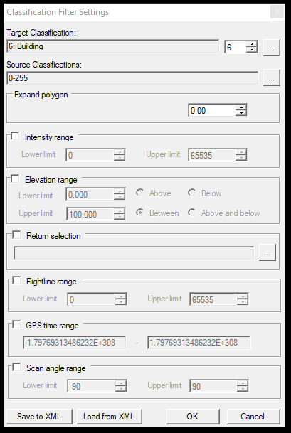
The description of the sections are the following:
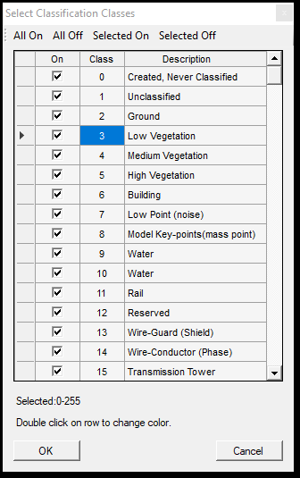
1. Source - Target classification - In these parts, the user can specify which class(es) shall be the points reclassified to which class. This is a multi-to-one selection, as multiple source classes can be selected, but only a single target class. The source and target classes can be selected by clicking the three points button and selecting the respective layers with the checkbox. The target class can be re-assigned with the counter as well.
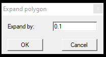
2. Expand Polygon - If a polygon is used for classification, the user can assign a buffer value for the polygon.
3. Intensity range - The intensity filter becomes active if the checkbox is selected. The user can filter the classification target for intensity range.
4. Elevation range - The elevation filter becomes active if the checkbox is selected. The user can specify a lower and upper elevation limit and decide if the software should update the classification above, below, in between, above and below the limits.
5. Return selection - The intensity filter becomes active if the checkbox is selected. The user can specify the return numbers that will be the classification target. Please note that this information might not be coded into the LAS file.
6. Flightline range - The flight line filter becomes active if the checkbox is selected. The user can specify which flight lines shall be targeted by the classification. Please note that this information might not be coded into the LAS file.
7. GPS time range - If the checkbox is selected, the GPS time range filter becomes active. The user can specify the GPS time range in which the classification shall be performed. Please note that this information might not be coded into the LAS file.
8. Scan angle range - If the checkbox is selected, the scan angle range filter becomes active. The user can specify the scan angle range in which the classification shall be performed. Please note that this information might not be coded into the LAS file.
9. Save to/Load from XML - Save the current setting to an XML file or load a previously saved setting.
Pressing OK will store the parameters, but as mentioned above, it will not perform any actions. Pressing Cancel will discard the changes.
- Class Dropdown menu - This menu contains classification tools that can be applied for all clouds or perform a batch re-classification task.
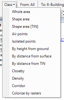
- Whole area - Performs a whole area re-classify - for all point clouds, which have all points in memory - based on the set classification filter settings. Starting the tool will open the classification filter settings - as described above. If the settings were previously modified, the modified settings will be visible. If the tool has been run before the last used settings, it will be stored until the software restarts. Pressing OK will act on all clouds. This might take a lot of time - depending on hardware and source data - and the software will seem stuck during the process.
- Shape area - Works the same as whole area classification, but the area of effect is only the active SHP's area. Starting the tool will open the classification filter settings window, but the active SHP shall be a polygon to start the function. The function will take all polygon areas in the active SHP so that multiple smaller parts can be re-classified simultaneously.
- Shape area [TIN] - Works the same as the Shape Area option with a slight difference: The software will interpolate a TIN surface from the polygon points and will reclassify only those points which are within +/- the set tolerance of the generated TIN.
- Air points - This function can filter air points, which can be dust or flying birds. After starting the tool, the settings window will appear.
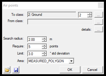
As usual, the user can pick the source and target classes in the settings window. Selecting the three dots next to the details text will bring up the classification filter settings window, where further parameters can be set. The search radius will specify how far each cloud point's environment shall be inspected, whether there are neighbouring points or not. If there are insufficient points, it means that it is an air point, and that point will be re-classified. The required point is a setting that will set how many points shall be minimally found within the search radius to avoid re-classification. The limit option will check the standard deviation of the points. The area of effect can be a measured polygon (2D drawn polygon just like selection commands), the active SHP (which can be polyline or polygon) or the whole area. The settings can be saved via the floppy icon and loaded with the load icon.
5. Isolated points - The isolated point filter works similarly to air points, but while air points can filter air objects like birds, this function will focus only on flying discrete points. After starting the function, the settings window will open:

As usual, the user can pick the source and target classes in the settings window. Selecting the three dots next to the details text will bring up the classification filter settings window, where further parameters can be set. The search radius will specify how far each cloud point's environment shall be inspected, whether there are neighbouring points or not. The "If fewer than" setting is set, a point is considered isolated if, within the search radius, fewer points can be found than the specified value. The area of effect can be a measured polygon (2D drawn polygon just like selection commands), the active SHP (which can be polyline or polygon) or the whole area. The settings can be saved via the floppy icon and loaded with the load icon.
6. By height from ground - This function can classify clouds above the ground class. If there is no ground class in the point cloud or it is of mediocre quality, we do not recommend using this function. The tool will take the ground class, generate a temporary TIN network in the background, and reclassify the points - according to the settings - above the ground surface. After starting the function, the settings window will open:
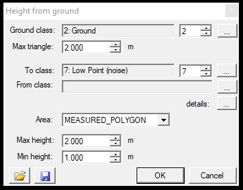
In the settings window, the first thing that should be set is the ground class. This is commonly class 2, but crosscheck the cloud classification by using the information tool from the Measure toolbar to be sure of the ground class. The ground class can be changed with the counter or by clicking the three dots. The max triangle will set the TIN's biggest triangle size. Before running the tool, consider the data type (SLAM, TLS, MLS, ALS) and select the respective TIN size. Choosing a smaller TIN might drastically increase processing time. In the next part, the user can pick the source and target classes as usual. Selecting the three dots next to the details text will bring up the classification filter settings window, where further parameters can be set. The area of effect can be a measured polygon (2D drawn polygon just like selection commands), the active SHP (which can be polyline or polygon) or the whole area. The user can specify minimum and maximum height (elevation). In that way, the classification can be forced into an elevation range. The settings can be saved via the floppy icon and loaded with the load icon.
7. By distance from surface - This function is similar to the previous By height from the ground, but the software will generate a surface from the designated class, which can be different from the ground class. After starting the function, the settings window will open:
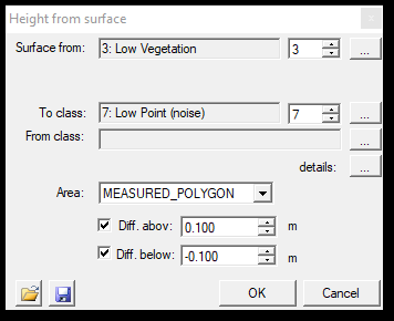
The first thing to be set in the settings window is the source class, from which the software will generate the surface. The source class can be changed with the counter or by clicking the three dots. In the next part, the user can pick the source and target classes as usual. Selecting the three dots next to the details text will bring up the classification filter settings window, where further parameters can be set. The area of effect can be a measured polygon (2D drawn polygon just like selection commands), the active SHP (which can be polyline or polygon) or the whole area. The user can specify the difference above or below the surface, creating a 3D buffer for the classification. The settings can be saved via the floppy icon and loaded with the load icon.
8. By distance from TIN - This function is similar to the previous By distance from the surface, but in this case, an active TRI file shall be used as a base for classification. The triangulated surface functionality is described in the respective article. The tool will re-classify the cloud against the triangulated surface. The tool can be started only if the active vector layer is a TRI file. After starting the function, the settings window will open:
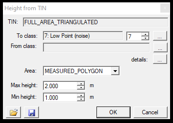
The first thing in the settings window is the active triangulated surface, which will be used for the process. In the next part, the user can pick the source and target classes as usual. Selecting the three dots next to the details text will bring up the classification filter settings window, where further parameters can be set. The area of effect can be a measured polygon (2D drawn polygon just like selection commands), the active SHP (which can be polyline or polygon) or the whole area. This function allows minimum and maximum height (elevation) to force the classification between an elevation range. The settings can be saved via the floppy icon and loaded with the load icon.
9. Closeby - This function allows the users to re-classify points close to another class by updating the source class. This allows the users to "buffer" a class. After starting the function, the settings window will open:
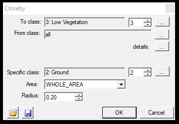
In the first part, the user can pick the source and target classes as usual. Selecting the three dots next to the details text will bring up the classification filter settings window, where further parameters can be set. The specific class is from which the software will interpolate the radius. The points in the radius will be reclassified, including the particular class points. The area of effect can be a measured polygon (2D drawn polygon just like selection commands), the active SHP (which can be polyline or polygon) or the whole area. The settings can be saved via the floppy icon and loaded with the load icon.
10. Density - This tool can be used to re-classify based on the source class' point density. This tool can be effectively used with the Measure Density tool from the Measure toolbar. After starting the function, the settings window will open:
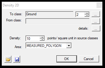
In the first part, the user can pick the source and target classes as usual. Selecting the three dots next to the details text will bring up the classification filter settings window, where further parameters can be set. At the density setting, the user can specify the number of points per square meter to be reclassified based on the source class. The area of effect can be a measured polygon (2D drawn polygon just like selection commands), the active SHP (which can be polyline or polygon) or the whole area. The settings can be saved via the floppy icon and loaded with the load icon.
11. Corridor - This tool can be used to re-classify points around pipes created by the pipe/corridor tool located at the Shape toolbar.
12. Colorize by raster - Assign RGB values for a point cloud based on the opened rasters currently in development.
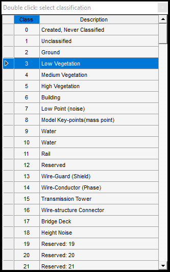
- From-To selectors - These selector fields allow the users to select the source and target classes for the classification. This is a global setting; it will also update this value in the class filter settings and the 3D window's classification toolbar. For the source class, multiple classes can be selected, for the target class only one.
- Modify by selected Shape - The tool allows the users to select a polygon element in the 2D view, and the points within the polygon will be re-classified based on the source-target class setting. The tool can be used only with an active polygon shape.
- Classify by measured polygon - This tool allows users to reclassify by a free-drawn polygon according to the current source-target class settings. The user can draw both in 2D and 3D view, but the software will evaluate the polygon in 2D view and classify every point in the whole elevation range which falls into the polygon. The user is not required to close the polygon; when the enter is pressed, the software will automatically connect the start and end points to close the polygon.
- Classify by measured polyline - This tool allows the users to draw a polyline, and the tool will re-classify around the polyline within a given buffer radius using the source-target class settings. After starting the tool, the user can draw 2D and 3D views, and when the enter button is pressed, the buffer window will appear, where the user can specify the buffer radius in meter dimension. The tool has a specific panel for quickly setting the source and target classes.
- Classify by fence - This tool allows users to reclassify with a "freehand" drawing, like drawing with the brush in paint. The user can freehand draw any shape in 2D view, and the software will automatically connect the start and end points. All points within the resulting polygon will be reclassified according to the source-target class settings. Using the profile mode setting, the tool will automatically reload the point cloud to the 3D window. The same logic applies as the point cloud also becomes "flat" in 3D view. If users are unfamiliar with the profile mode, please read the clip frame toolbar article.
- Classify by brush - This tool allows users to use a "brush" to reclassify points according to the source-target settings. The previous tool allowed the user to free-hand a polygon, and everything inside would be reclassified. This tool will reclassify only the area included in the brush's drawn area. After starting the tool, the setting panel will appear:
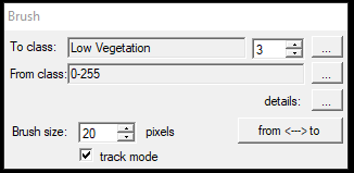
In the first part, the user can pick the source and target classes as usual. Selecting the three dots next to the details text will bring up the classification filter settings window, where further parameters can be set. Below the source-target settings, the brush size can be set in pixels. This brush is zoom-independent, which means it remains 20 pixels on the 1:10 scale and the 1:1000 scale, making it easy to adjust the size by zooming in and out. The tool, by default, allows the users to draw a 2-point line, and the given pixel range will be re-classified between the two points. However, if the user turns on track mode, the tool becomes a free-hand brush, as the user would use it in a colouring book. This is useful for fine-detail classification, such as training data annotation for ML engines. The from and to button is currently a blind button. Using the profile mode setting, the tool will automatically reload the point cloud to the 3D window. As the point cloud also becomes "flat" in 3D view, the same logic applies there. If users are unfamiliar with the profile mode, please read the article on clip frame toolbars.
- Reclassify by point - This tool allows the user to re-classify points individually. This tool might seem odd as we work with enormous datasets, but in some cases, tiny point clouds can be used (for example, a point cloud generated from vectors). After starting the tool, the classification filter settings will be opened. The user can adjust the settings here before beginning the classification itself. After the OK button is pressed, the tool will take the first point and open a new information window.
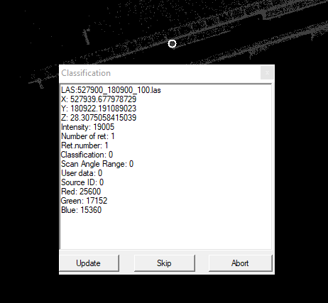
At the information panel, all information about the point can be seen. Pressing the update button will result in the source-target classification setting will be applied to the point. Pressing the skip will jump to the next point. Pressing abort will close the operation. After pressing abort, the tool will ask if the points should be inspected against the classification filter settings. Press No, as it has been already taken into account, this is a redundant question.
- Undo classification - Undo the last classification operation. The function is unavailable until at least one classification operation has been performed. The software cannot store an unlimited amount of undo operations for classifications. Please read the classification article for a better understanding. This undo is not related in any way to vector undo located at the shape toolbar.
- Undo more - This function allows the users to undo multiple operations. After starting the tool, a window will appear where the user can see the latest classification actions, including their settings, the number of points reclassified and the time taken.
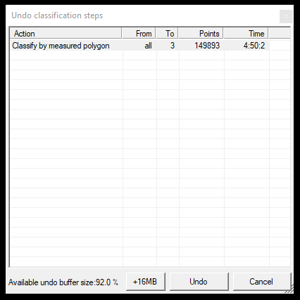
The remaining buffer size in this window can also be seen at the bottom. If the buffer gets full, the user either clears the buffer (from that point, the previous classification operations cannot be undone) or increases the buffer size, which can also be performed in this window.
- Clear Undo - Clear the undo list and buffer memory for the classification operations. It does not affect vector undo operations.
- Create Popup - The function will place a Classification menu on the top bar after the Help menu so that the tools can be accessed from the menu until the software restarts.